To begin, load the interpretnn package.
Also, load the package that we will use to fit the neural network.
Our package works with a number of popular R packages for neural
networks, and here we will use the nnet package.
Now, load the data.
# load data ---------------------------------------------------------------
data(Boston)
Next, we fit a neural network. We will fit a neural network on the
respose variable, medv, using all covariates and with two
hidden nodes. As neural networks require random initial weights to begin
learning, we use set.seed() for reproducibility.
set.seed(100)
nn <- nnet(medv ~ ., data = Boston, size = 2, trace = FALSE,
           linout = TRUE, maxit = 1000)
We can then create a interpretnn object
intnn <- interpretnn(nn, X = Boston[, -ncol(Boston)]) A useful summary table can then be produced using the
summary() function
summary(intnn)
#> Call (interpretnn):
#> interpretnn.nnet(object = ..1, X = ..2)
#>
#> Number of input nodes: 12
#> Number of hidden nodes: 2
#>
#> BIC: 606.4537
#>
#> Coefficients:
#>                                        Wald
#>          Estimate Std. Error |       X^2    Pr(> X^2)
#>     crim -0.50367   0.080639 |  15.86103 3.60e-04 ***
#>       zn  0.89640   0.084741 |   7.13194 2.83e-02 *
#>    indus -0.85112   0.074677 |   0.10822 9.47e-01
#>     chas  0.71421   0.199555 |   8.12925 1.72e-02 *
#>      nox -0.71383   0.080419 |  16.20045 3.03e-04 ***
#>       rm  0.94949   0.071141 | 102.72926 0.00e+00 ***
#>      age -0.70553   0.079025 |   1.54725 4.61e-01
#>      dis  0.58585   0.089845 |  39.16725 3.13e-09 ***
#>      rad -0.48035   0.089325 |  41.56443 9.43e-10 ***
#>      tax -0.76588   0.083371 |  10.40137 5.51e-03 **
#>  ptratio -0.93611   0.071849 |  19.46303 5.94e-05 ***
#>    lstat -1.27902   0.061575 |  59.52595 1.19e-13 ***
#> ---
#> Signif. codes:  0 '***' 0.001 '**' 0.01 '*' 0.05 '.' 0.1 ' ' 1
#>
#> Weights:
#>      b0->h11    crim->h11      zn->h11   indus->h11    chas->h11     nox->h11
#>        -2.19        -0.14         0.13        -0.03         0.06         0.15
#>      rm->h11     age->h11     dis->h11     rad->h11     tax->h11 ptratio->h11
#>         0.74        -0.05        -0.35         0.99        -0.13        -0.16
#>   lstat->h11      b0->h12    crim->h12      zn->h12   indus->h12    chas->h12
#>        -1.38         6.58        -0.52        10.13         0.00         0.12
#>     nox->h12      rm->h12     age->h12     dis->h12     rad->h12     tax->h12
#>        -1.42        -0.88        -0.20        -1.85         0.31        -1.14
#> ptratio->h12   lstat->h12        b1->y       h11->y       h12->y
#>        -0.66        -0.69        -1.83         3.61         1.50
This tells provides us with simple point estimates of the effects, and the results from the multiple-parameter Wald test for each input.
We can visualise the covariate effects and their associated
uncertainty using the plot() function, which creates
Partial Covariate Effect (PCE) plots.
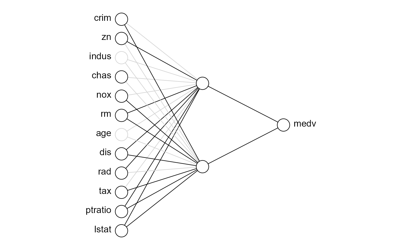
There is also a plotnn() function that visualise the
significance of each weight from the single-parameter Wald test.
plotnn(intnn)